Deep Learning: Meta Learning
The purpose of machine learning is to create algorithms that make accurate predictions on input data. For example, your new social network for pets may need an algorithm to detect whether a profile picture shows a cat or a dog.

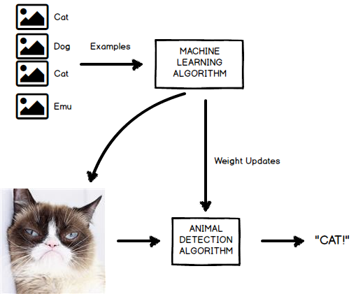
Figure 1: An algorithm that tells you what animal is in the picture
You could go ahead and write a complex algorithm that detects fur, whiskers, ears and paws, and glue those together to determine what animal is in a picture. That would not be machine learning however. No, in machine learning, the animal detection algorithm has to be generated by a second algorithm, which should learn from examples how to write the animal detector for us.

Figure 2: An algorithm that creates an animal detection algorithm by looking at many examples of animals
There is lots of research being done on how to create the best machine learning to do this. Today, when you are tasked with distinguishing cats from dogs in a picture, you would probably choose to use a convolutional neural net such as AlexNet, or maybe a ResNet, and use gradient descent to optimize the parameters of this model. This is an approach that works well for picture classification, assuming you have thousands of example pictures labeled with dog/cat classifications. Techniques such as convolutional nets are domain specific. Convolutional nets work great for classifying pictures, but don’t help you predict future stock prices or the topic of tweets.
The question meta learning brings up is the following. Instead of focusing on creating great machine learning algorithms for domain specific use cases, could we not have another machine learning algorithm do that for us? In other words, could we have another machine learning algorithm learn how to create machine learning algorithms for us? That is what we call meta learning.
The Idea of Meta Learning
Convolutional neural nets work great for classifying images. The reason we know that is because researchers have compared and contrasted many different machine learning architectures on popular image datasets such as CIFAR (tiny pictures of airplanes, birds, cats, etc) and MNIST (written digits). The architecture of Convolutional neural nets exploits the fact that images are two dimensional, and that adjacent pixels in an image have a special relation to each other. In essence, there is a commonality between the tasks of classifying images that a convolutional net is particularly tuned to. That special tuning gives them their superior accuracy. This ‘tuning’ effect is what we want to imitate in a meta learning algorithm.
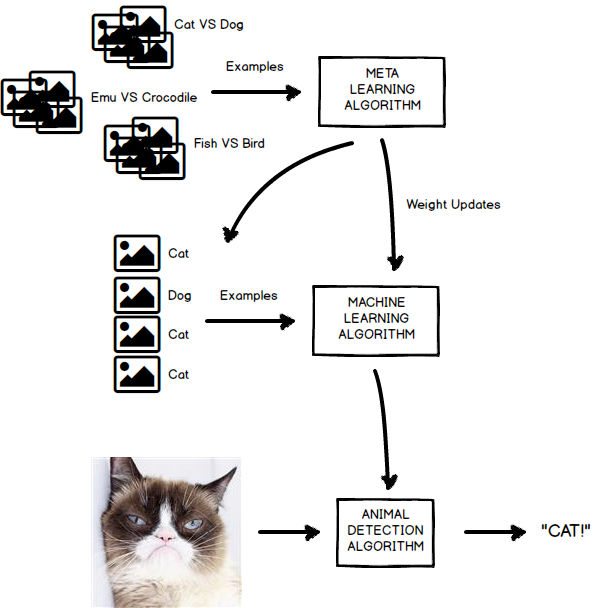
 Figure 3: An algorithm that learns to make machine learning algorithms that make animal detection algorithms
In meta learning, we want a ‘master’ machine learning algorithm to generate machine learning algorithm specifically tuned to one specific task. This is not a trivial thing to do. A first attempt may be to use some type of automated code generation and run it. Maybe you could even bake in popular kernels, convolutions, and optimization methods, and combine them in creative ways. This is possible, you could try that. Your algorithm would essentially create a machine learning program, would run it, and then it’d check how fast and well it learned to detect cats and dogs, and change it’s algorithm depending on some performance metric. There is, however, one big downside to such approach, and that is that it is not differentiable. In order to optimize a non-differentiable system you would have to resort to evolutionary algorithms, genetic programming and the likes. Wouldn’t it be great if we could use the same deep learning algorithms with gradient descent that bring so much success in other tasks instead? A way to do this was proposed by Hochreiter back in 2001 in his paper Learning to Learn Using Gradient Descent.
Meta Learning using RNNs
Instead of generating code, or lines of logic, to create candidate machine learning algorithms, the machine learning algorithm itself could be constructed in the form of a Recurrent Neural Network (RNN). In essence, you can ‘program’ an RNN by setting it’s weights. If we set up the meta learning system in this way, the result is that the machine learning algorithm itself can be optimized with gradient descent!
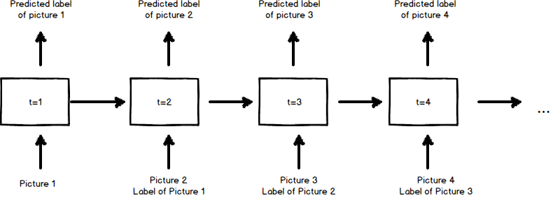
 Figure 4: A rolled out RNN that represents a machine learning algorithm
Let’s take a look at how this works. At each timestep of the RNN, the meta learning algorithm will feed the RNN one example picture together with the correct label for the previous example picture. The output of the RNN at each timestep is the predicted label of the current example picture (the reason why the correct labels are inputted one time step after the image is to prevent the RNN from cheating; it could just output the correct answer immediately without learning anything). The meta learning algorithm will use gradient descent to update the weights of the RNN based on the accuracy of the labels it predicts. It is interesting to note that at this time we have no clear idea of how the weights of the RNN actually execute the machine learning algorithm.
Performance
The performance of meta learning using RNNs has been quite amazing. Below are some examples.
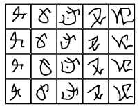
One-shot Learning with Memory-Augmented Neural Networks (2016) In this paper, the authors contributed a clever extension of Neural Turing Machines (NTM), which itself is a combination of LSTMs with a memory module. The algorithm is tested on the Omniglot dataset. The Omniglot dataset contains 1623 different handwritten characters from 50 different alphabets. Each character has about 20 samples in total. They train the meta learning algorithm on 1200 types of characters, and then apply it on a holdout set of 423 classes. The resulting machine learning algorithm is able to successfully classify characters with 94.9% accuracy after only 5 samples, and 98.1% accuracy after only 10 samples! Compare this with convolutional neural networks that require thousands of samples per class to even work in the first place.
 Figure 5: Omniglot dataset example
Learning to Learn Using Gradient Descent (2001) Hochreiter shows that a simple LSTM can be used to learn to approximate any quadratic function after only 35 examples.